Reinforcement learning,
A path to machine control,
Through trial and error,
Optimizing the goal.

Rewards guide the way
A signal to the brain,
A system to improve,
A future to gain.

But, the journey is long,
And the road is steep,
Only the strong survive,
To reach the final leap.

So, let us strive,
To make our algorithms thrive,
Through reinforcement learning,
We'll make machines come alive.

Thank you, ChatGPT for this cute poem! Although, I’m not really sure how I feel about the last line haha.

I decided to tackle some reinforcement learning exercises that I found in my textbook, and think I might make this a several part series. Although I have a summer’s worth of reinforcement learning experience, I kind of jumped right into it and skipped over all of the basics. It’s worthwhile to formally introduce myself to some of these concepts. So let’s get into it:

First, I’m not sure if anyone else has this problem, but I could spend hours trying to figure out why certain packages aren’t installing on my local computer. I think from now on if I have to use anything besides numpy, I’ll go to Google Colab.

In this first part, we make sure that all of the required libraries are installed and up to date, make sure our plots will be nicely formatted, animations can be made and figures saved— I’m in a rhyming mood :)

Setup and Intro to OpenAI gym

# Python ≥3.5 is required
import sys
assert sys.version_info >= (3, 5)

# Is this notebook running on Colab?
IS_COLAB = "google.colab" in sys.modules


if IS_COLAB or IS_KAGGLE:
    !apt update && apt install -y libpq-dev libsdl2-dev swig xorg-dev xvfb
    %pip install -U tf-agents pyvirtualdisplay
    %pip install -U gym~=0.21.0
    %pip install -U gym[box2d,atari,accept-rom-license]

# Scikit-Learn ≥0.20 is required
import sklearn
assert sklearn.__version__ >= "0.20"

# TensorFlow ≥2.0 is required
import tensorflow as tf
from tensorflow import keras
assert tf.__version__ >= "2.0"

if not tf.config.list_physical_devices('GPU'):
    print("No GPU was detected. CNNs can be very slow without a GPU.")
    if IS_COLAB:
        print("Go to Runtime > Change runtime and select a GPU hardware accelerator.")

# Common imports
import numpy as np
import os

# to make this notebook's output stable across runs
np.random.seed(42)
tf.random.set_seed(42)

# To plot pretty figures
%matplotlib inline
import matplotlib as mpl
import matplotlib.pyplot as plt
mpl.rc('axes', labelsize=14)
mpl.rc('xtick', labelsize=12)
mpl.rc('ytick', labelsize=12)

# To get smooth animations
import matplotlib.animation as animation
mpl.rc('animation', html='jshtml')

# Where to save the figures
PROJECT_ROOT_DIR = "."
CHAPTER_ID = "rl"
IMAGES_PATH = os.path.join(PROJECT_ROOT_DIR, "images", CHAPTER_ID)
os.makedirs(IMAGES_PATH, exist_ok=True)

def save_fig(fig_id, tight_layout=True, fig_extension="png", resolution=300):
    path = os.path.join(IMAGES_PATH, fig_id + "." + fig_extension)
    print("Saving figure", fig_id)
    if tight_layout:
        plt.tight_layout()
    plt.savefig(path, format=fig_extension, dpi=resolution)

import gym

First we are going to create an environment with make():
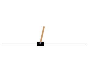
For this example we are going to use the CartPole environment. This is a 2D simulation with a pole balanced on a cart.

env = gym.make('CartPole-v1',render_mode="rgb_array")

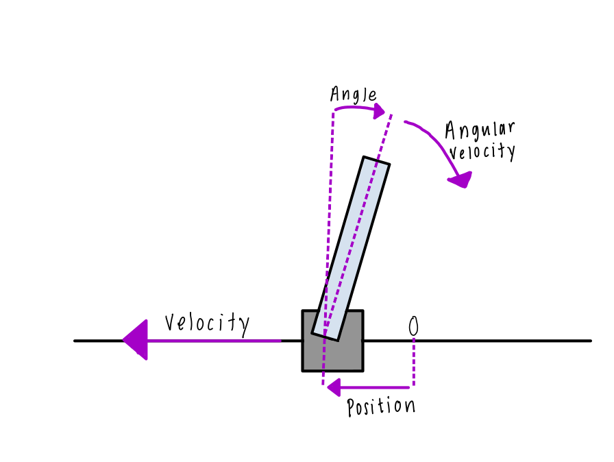
Initialize the environment using reset(). Returned is the first set of observations. For the CartPole environment, the observations of are the following four:

Cart’s horizontal position (0.0 = center)
Cart’s velocity (>0 = right)
Pole’s angle (0.0 = vertical)
Pole’s angular velocity (>0 = clockwise)

obs = env.reset()

env.np_random.random(32)
obs

array([-0.2303003 , -0.9796561 , 0.21622495, 1.1510738 ], dtype=float32)

try:
  import pyvirtualdisplay
  display = pyvirtualdisplay.Display(visible=0, size=(1400, 900)).start()
  print('worked')
except ImportError:
  pass

Use the render() function to show the environment.

img = env.render()

img.shape

(400, 600, 3)

def plt_env(env):
  plt.figure(figsize=(5,4))
  img = env.render()
  plt.imshow(img)
  plt.axis("off")
  return img 

plt_env(env)
plt.show()

env.action_space() shows which actions are possible in the environment. Discrete(2) means that there are two possible actions that the agent can take: 0 (accelerating left) or 1 (accelerating right).

env.action_space

Discrete(2)

Just as an example, let’s accelerate the cart to the left by setting action = 0. The step() function executes the action and returns four values:

obs: The newest observation. If we compare the two angular velocities obs[2] we will see that it increases, which means the pole is moving to the right, as we expect it to!
reward: We want the episode to run for as long as possible, so we set the reward to 1 at each step.
done: When the episode is over, done will be equal to TRUE. This will happen either when the angle of the pole falls below 0 (which means it falls off the screen) or we reach the end of the 200 steps, which means we have won.
info: This provides extra information for training or debugging.

I am imagining that episodes in this context are akin to epochs. After going through all of the steps per epoch, the environment is reset and the agent’s reward is set to 0.

action = 0
stats=env.step(action)
obs = stats[0]
reward = stats[1]
done = stats[2]
info = stats[3]

plt_env(env)
plt.show()

save_fig("cart_pole_plot")

Saving figure cart_pole_plot

<Figure size 432x288 with 0 Axes>

print(obs)
print(reward)
print(done)
print(info)

[-0.2303003 -0.9796561 0.21622495 1.1510738 ]
1.0
True
False

if done:
  obs = env.reset()

To demonstrate how this works all together, let’s create a simple hard-coded policy that will accelerate the cart to the left when the pole is leaning towards and accelerate it to the right when the pole is leaning right.

Creating a Simple-Hardcoded Policy

def basic_policy(obs):
  angle = obs[2]
  return 0 if angle < 0 else 1 

import array
from numpy.core.memmap import dtype

env.np_random.random(32)
totals=[] 

for episode in range(500):
  episode_rewards = 0 
  obs = env.reset()
  obs = np.array(obs[0])

  for step in range(200):
    #action will either be 0 or 1 
    action = basic_policy(obs)
    #get all information from each action 
    stats = env.step(action)
    obs = np.array(stats[0])
    reward = stats[1]
    done = stats[2]
    info = stats[3]

    episode_rewards += reward 

    if done: 
       break
       
  totals.append(episode_rewards) 

print('mean',np.mean(totals) ,np.std(totals),np.min(totals),np.max(totals))

The max value indicates that out of 500 tries, the pole managed to stay upright for 72 consecutive steps.

mean: 42.992
std: 8.717105941767601
min: 24.0
max: 72.0

Visualization

env.np_random.random(32)

frames = [] 

obs = env.reset()
obs = np.array(obs[0])
for step in range(200):
  img = env.render()
  frames.append(img)
  action = basic_policy(obs)

  stats=env.step(action)
  obs = np.array(stats[0])
  reward = stats[1]
  done = stats[2]
  info = stats[3]

  if done: 
    break

def update_scene(num,frames,patch): 
  patch.set_data(frames[num])
  return patch

def plot_animation(frames,repeat=False,interval=40):
  fig = plt.figure()
  patch = plt.imshow(frames[0])
  plt.axis('off')
  anim = animation.FuncAnimation(fig,update_scene, fargs=(frames,patch),
                                 frames=len(frames),repeat=repeat,interval=interval)
  
  plt.close()
  return anim 

plot_animation(frames)

</input>

We can see from the animation that over the course of one episode the pole increasingly tilts more to the left and right. Eventually it would fall out of frame.

Let’s try using a neural network policy in the next segment (which will prob be in a few days)! Byeee.