Feature Engineering for Alpha Factor Research
Alpha factors are mathematical expressions or models that aim to quantify the skill of an investment strategy in generating excess returns beyond what would be expected given the associated risks i.e. it represents the active return of a portfolio.
Here is the data that we are going to use:
The wiki prices is a NASDAQ dataset that has stock prices, dividends, and splits for 3000 US publicly-traded companies wiki prices data
The US Equities Meta-Data can be found on my github. Beware it is a large file ~1.8 GB. us equities meta data
Imports
%pip install pandas_datareader
%pip install statsmodels
import warnings
warnings.filterwarnings('ignore')

import pandas as pd
import pandas_datareader.data as web

import seaborn as sns

from statsmodels.regression.rolling import RollingOLS

import statsmodels.api as sm

from datetime import datetime
START = 2000
END = 2018

idx = pd.IndexSlice
Read and Store Data
# parse prices data

df_prices = (pd.read_csv('WIKI_PRICES.csv',
                 parse_dates = ['date'],
                 index_col = ['date','ticker'],
                 infer_datetime_format=True)).sort_index()

df_screener = pd.read_csv('us_equities_meta_data.csv')
# store price and stock data

with pd.HDFStore('assets.h5') as store:
    store.put('data_prices',df_prices)
    store.put('data_screener',df_screener)
# read in prices and stocks
'''
get all the dates between START and END and
then get the adj_close column
reshape df by turning the tickers into the columns and have the adj value for every date
we convert the rows into columns so that we can easily access the tickers later on
'''


with pd.HDFStore('assets.h5') as store:
    prices = (store['data_prices']
              .loc[idx[str(START):str(END), :], 'adj_close']
              .unstack('ticker'))
    stocks = store['data_screener'].loc[:, ['ticker','marketcap', 'ipoyear', 'sector']]
prices.info()
<class 'pandas.core.frame.DataFrame'>
DatetimeIndex: 4706 entries, 2000-01-03 to 2018-03-27
Columns: 3199 entries, A to ZUMZ
dtypes: float64(3199)
memory usage: 114.9 MB
stocks.info()
<class 'pandas.core.frame.DataFrame'>
Int64Index: 6834 entries, 0 to 6833
Data columns (total 4 columns):
 #   Column     Non-Null Count  Dtype
---  ------     --------------  -----
 0   ticker     6834 non-null   object
 1   marketcap  5766 non-null   float64
 2   ipoyear    3038 non-null   float64
 3   sector     5288 non-null   object
dtypes: float64(2), object(2)
memory usage: 267.0+ KB
Data Cleaning
remove stock duplicates and reset the index name for later data manipulation
stocks = stocks[~stocks.index.duplicated()]
stocks = stocks.set_index('ticker')
get all of the common tickers with their price information and metadata
shared = prices.columns.intersection(stocks.index)
stocks = stocks.loc[shared, :]
stocks.info()
<class 'pandas.core.frame.DataFrame'>
Index: 2412 entries, A to ZUMZ
Data columns (total 3 columns):
 #   Column     Non-Null Count  Dtype
---  ------     --------------  -----
 0   marketcap  2407 non-null   float64
 1   ipoyear    1065 non-null   float64
 2   sector     2372 non-null   object
dtypes: float64(2), object(1)
memory usage: 75.4+ KB
prices = prices.loc[:, shared]
prices.info()
<class 'pandas.core.frame.DataFrame'>
DatetimeIndex: 4706 entries, 2000-01-03 to 2018-03-27
Columns: 2412 entries, A to ZUMZ
dtypes: float64(2412)
memory usage: 86.6 MB
assert prices.shape[1] == stocks.shape[0]
Create a Monthly Return Series
monthly_prices = prices.resample('M').last()
monthly_prices.info()
<class 'pandas.core.frame.DataFrame'>
DatetimeIndex: 219 entries, 2000-01-31 to 2018-03-31
Freq: M
Columns: 2412 entries, A to ZUMZ
dtypes: float64(2412)
memory usage: 4.0 MB
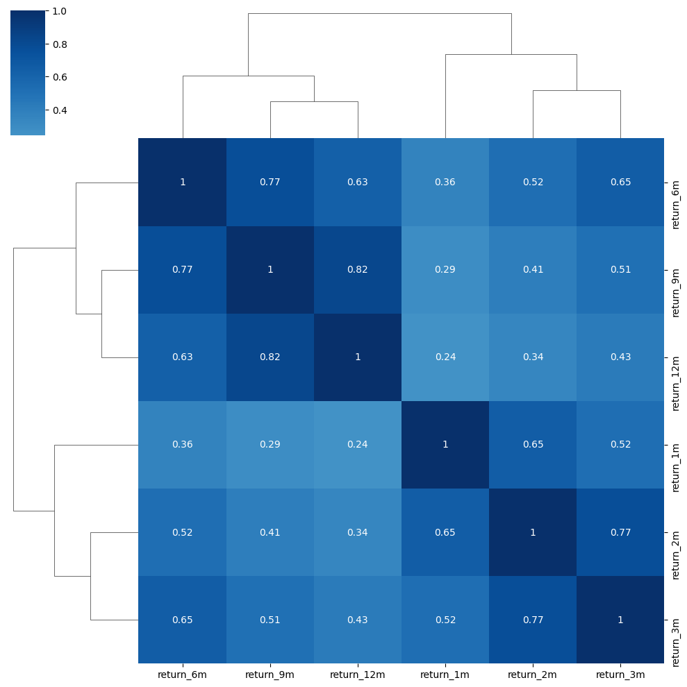
Here, we calculate the precentage change of monthly prices over a lag period. This represents the return over the specified number of months.
Clip outliers in the data based on the outlier_cutoff quantile and the 1- outlier_cutoff to their respective quantile values. Add 1 to the clipped values. This is to handle returns and convert percentage changes back to absolute returns.
Raise each value to the power of \(\frac{1}{lag}\). This is used to annualize returns when the lag is representative of months.
outlier_cutoff = 0.01
data = pd.DataFrame()
lags = [1, 2, 3, 6, 9, 12]
for lag in lags:
    data[f'return_{lag}m'] = (monthly_prices
                           .pct_change(lag)
                           .stack()
                           .pipe(lambda x: x.clip(lower=x.quantile(outlier_cutoff),
                                                  upper=x.quantile(1-outlier_cutoff)))
                           .add(1)
                           .pow(1/lag)
                           .sub(1)
                           )
data = data.swaplevel().dropna()
data.info()
<class 'pandas.core.frame.DataFrame'>
MultiIndex: 399525 entries, ('A', Timestamp('2001-01-31 00:00:00', freq='M')) to ('ZUMZ', Timestamp('2018-03-31 00:00:00', freq='M'))
Data columns (total 6 columns):
 #   Column      Non-Null Count   Dtype
---  ------      --------------   -----
 0   return_1m   399525 non-null  float64
 1   return_2m   399525 non-null  float64
 2   return_3m   399525 non-null  float64
 3   return_6m   399525 non-null  float64
 4   return_9m   399525 non-null  float64
 5   return_12m  399525 non-null  float64
dtypes: float64(6)
memory usage: 19.9+ MB
Drop Stocks with Less than 10 Years of Returns
min_obs = 120

# get the number of observations for each ticker
nobs = data.groupby(level='ticker').size()

# get the indices of the tickers where the num of observations is greater than min_obs
keep = nobs[nobs>min_obs].index

# get the data with appropriate tickers and their respective data
data = data.loc[idx[keep,:], :]
data.info()
<class 'pandas.core.frame.DataFrame'>
MultiIndex: 360752 entries, ('A', Timestamp('2001-01-31 00:00:00', freq='M')) to ('ZUMZ', Timestamp('2018-03-31 00:00:00', freq='M'))
Data columns (total 6 columns):
 #   Column      Non-Null Count   Dtype
---  ------      --------------   -----
 0   return_1m   360752 non-null  float64
 1   return_2m   360752 non-null  float64
 2   return_3m   360752 non-null  float64
 3   return_6m   360752 non-null  float64
 4   return_9m   360752 non-null  float64
 5   return_12m  360752 non-null  float64
dtypes: float64(6)
memory usage: 18.0+ MB
data.describe()
| return_1m | return_2m | return_3m | return_6m | return_9m | return_12m | |
|---|---|---|---|---|---|---|
| count | 360752.000000 | 360752.000000 | 360752.000000 | 360752.000000 | 360752.000000 | 360752.000000 |
| mean | 0.012255 | 0.009213 | 0.008181 | 0.007025 | 0.006552 | 0.006296 |
| std | 0.114236 | 0.081170 | 0.066584 | 0.048474 | 0.039897 | 0.034792 |
| min | -0.329564 | -0.255452 | -0.214783 | -0.162063 | -0.131996 | -0.114283 |
| 25% | -0.046464 | -0.030716 | -0.023961 | -0.014922 | -0.011182 | -0.009064 |
| 50% | 0.009448 | 0.009748 | 0.009744 | 0.009378 | 0.008982 | 0.008726 |
| 75% | 0.066000 | 0.049249 | 0.042069 | 0.031971 | 0.027183 | 0.024615 |
| max | 0.430943 | 0.281819 | 0.221789 | 0.154555 | 0.124718 | 0.106371 |
sns.clustermap(data.corr('spearman'), annot=True, center=0, cmap='Blues');
data.index.get_level_values('ticker').nunique()
1838
Rolling Factor Betas
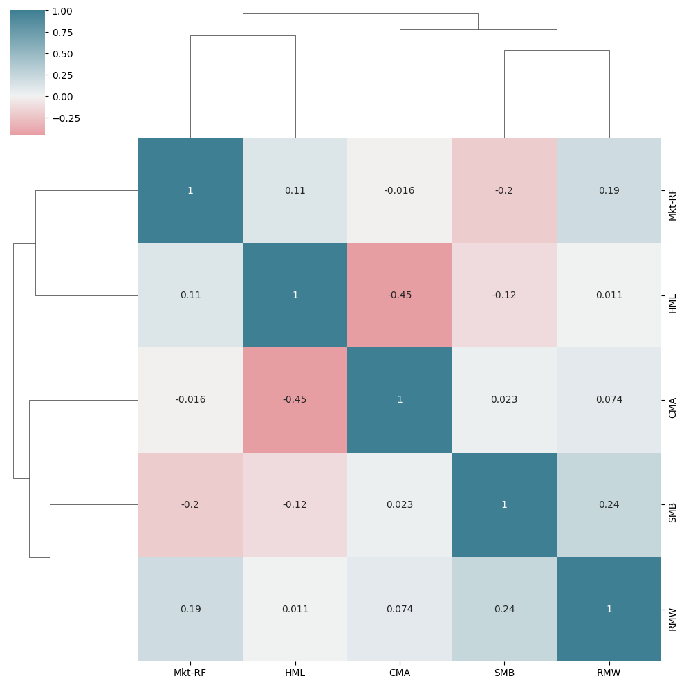
In this section we are going to estimate the factor exposure of the listed stocks in the database according to the Fama-French Five-Factor Model.
Mkt-Rf is the market risk premium \((R_m - R_f)\). The difference between these two factors represents the additional return investors demand for bearing the systemic risk associated with the market.
SMB is small minus big. This factor represents the spread between small-cap and large-cap stocks.
SMB is typically measured in terms of market capitalization which is represented as \(MarketCapitalization = currentStockPrice * TotalNumberOfOutstandingShares\)
HML is high minus low, which is the spread between high book-to-market and low book-to-market stocks. The book-to-market ratio is \(\frac{shareholder'sEquity}{marketCapitalization}\).
RMW is robust minus weak. This compares the returns of firms with higher operating profitability and those with weak operating probitability
CMA is conservative minus aggressive and it gauges the difference between companies that invest aggressively and those that do so more conservatively.
factors = ['Mkt-RF', 'SMB', 'HML', 'RMW', 'CMA']
factor_data = web.DataReader('F-F_Research_Data_5_Factors_2x3', 'famafrench', start='2000')[0].drop('RF', axis=1)
factor_data.index = factor_data.index.to_timestamp()
factor_data = factor_data.resample('M').last().div(100)
factor_data.index.name = 'date'
factor_data.info()
<class 'pandas.core.frame.DataFrame'>
DatetimeIndex: 289 entries, 2000-01-31 to 2024-01-31
Freq: M
Data columns (total 5 columns):
 #   Column  Non-Null Count  Dtype
---  ------  --------------  -----
 0   Mkt-RF  289 non-null    float64
 1   SMB     289 non-null    float64
 2   HML     289 non-null    float64
 3   RMW     289 non-null    float64
 4   CMA     289 non-null    float64
dtypes: float64(5)
memory usage: 13.5 KB
factor_data = factor_data.join(data['return_1m']).sort_index()
factor_data.info()
<class 'pandas.core.frame.DataFrame'>
MultiIndex: 360752 entries, ('A', Timestamp('2001-01-31 00:00:00', freq='M')) to ('ZUMZ', Timestamp('2018-03-31 00:00:00', freq='M'))
Data columns (total 6 columns):
 #   Column     Non-Null Count   Dtype
---  ------     --------------   -----
 0   Mkt-RF     360752 non-null  float64
 1   SMB        360752 non-null  float64
 2   HML        360752 non-null  float64
 3   RMW        360752 non-null  float64
 4   CMA        360752 non-null  float64
 5   return_1m  360752 non-null  float64
dtypes: float64(6)
memory usage: 18.0+ MB
Unlike traditional linear regression that considers an entire dataset, rolling linear regression calculates regresion coefficients and other statistics for a specified window of consecutive data points and then moves a window forward one observation at a time. Rolling Linear Regression is helpful when delaing with non-stationary time series data.
T = 24
betas = (factor_data.groupby(level='ticker',
                             group_keys=False)
         .apply(lambda x: RollingOLS(endog=x.return_1m,
                                     exog=sm.add_constant(x.drop('return_1m', axis=1)),
                                     window=min(T, x.shape[0]-1))
                .fit(params_only=True)
                .params
                .drop('const', axis=1)))
betas.describe().join(betas.sum(1).describe().to_frame('total'))
| Mkt-RF | SMB | HML | RMW | CMA | total | |
|---|---|---|---|---|---|---|
| count | 318478.000000 | 318478.000000 | 318478.000000 | 318478.000000 | 318478.000000 | 360752.000000 |
| mean | 0.979365 | 0.626588 | 0.122610 | -0.062073 | 0.016754 | 1.485997 |
| std | 0.918116 | 1.254249 | 1.603524 | 1.908446 | 2.158982 | 3.306487 |
| min | -9.805604 | -10.407516 | -15.382504 | -23.159702 | -18.406854 | -33.499590 |
| 25% | 0.463725 | -0.118767 | -0.707780 | -0.973586 | -1.071697 | 0.000000 |
| 50% | 0.928902 | 0.541623 | 0.095292 | 0.037585 | 0.040641 | 1.213499 |
| 75% | 1.444882 | 1.304325 | 0.946760 | 0.950267 | 1.135600 | 3.147199 |
| max | 10.855709 | 10.297453 | 15.038572 | 17.079472 | 16.671709 | 34.259432 |
cmap = sns.diverging_palette(10,220,as_cmap=True)
sns.clustermap(betas.corr(),annot=True,cmap=cmap,center=0);
data = (data.join(betas.groupby(level='ticker').shift()))
data.info()
<class 'pandas.core.frame.DataFrame'>
MultiIndex: 360752 entries, ('A', Timestamp('2001-01-31 00:00:00', freq='M')) to ('ZUMZ', Timestamp('2018-03-31 00:00:00', freq='M'))
Data columns (total 11 columns):
 #   Column      Non-Null Count   Dtype
---  ------      --------------   -----
 0   return_1m   360752 non-null  float64
 1   return_2m   360752 non-null  float64
 2   return_3m   360752 non-null  float64
 3   return_6m   360752 non-null  float64
 4   return_9m   360752 non-null  float64
 5   return_12m  360752 non-null  float64
 6   Mkt-RF      316640 non-null  float64
 7   SMB         316640 non-null  float64
 8   HML         316640 non-null  float64
 9   RMW         316640 non-null  float64
 10  CMA         316640 non-null  float64
dtypes: float64(11)
memory usage: 39.8+ MB
Impute Mean for Missing Factor Betas
data.loc[:, factors] = data.groupby('ticker')[factors].apply(lambda x: x.fillna(x.mean()))
data.info()
<class 'pandas.core.frame.DataFrame'>
MultiIndex: 360752 entries, ('A', Timestamp('2001-01-31 00:00:00', freq='M')) to ('ZUMZ', Timestamp('2018-03-31 00:00:00', freq='M'))
Data columns (total 11 columns):
 #   Column      Non-Null Count   Dtype
---  ------      --------------   -----
 0   return_1m   360752 non-null  float64
 1   return_2m   360752 non-null  float64
 2   return_3m   360752 non-null  float64
 3   return_6m   360752 non-null  float64
 4   return_9m   360752 non-null  float64
 5   return_12m  360752 non-null  float64
 6   Mkt-RF      360752 non-null  float64
 7   SMB         360752 non-null  float64
 8   HML         360752 non-null  float64
 9   RMW         360752 non-null  float64
 10  CMA         360752 non-null  float64
dtypes: float64(11)
memory usage: 39.8+ MB
Momentum Factors
Momentum represents the speed or velocity in which prices change in a publicly traded security. Momentum is caluclated by taking the return of the equal weighted average of the 30% highest performing stocks minus the return of the equal weighted average of the 30% lowest performing stocks.
Here, we create multiple momentum factors based on different lag periods and an additional momentum factor based on the difference between the 12 month and 3 month returns.
for lag in [2,3,6,9,12]:
    # for each value in the loop, calculate new column
    # momentum is computed as the difference between the return for that lag period
    # and the reutrn for the most recent month
    data[f'momentum_{lag}'] = data[f'return_{lag}m'].sub(data.return_1m)

data[f'momentum_3_12'] = data[f'return_12m'].sub(data.return_3m)
Date Indicators
# date indicators

dates = data.index.get_level_values('date')
data['year'] = dates.year
data['month'] = dates.month
Lagged Returns
# to use lagged values as input variables or features associated with the current observations
# we use the shift function to move historical returns up to the current period

for t in range(1,7):
    data[f'return_1m_t-{t}'] = data.groupby(level='ticker').return_1m.shift(t)
data.info()
<class 'pandas.core.frame.DataFrame'>
MultiIndex: 360752 entries, ('A', Timestamp('2001-01-31 00:00:00', freq='M')) to ('ZUMZ', Timestamp('2018-03-31 00:00:00', freq='M'))
Data columns (total 25 columns):
 #   Column         Non-Null Count   Dtype
---  ------         --------------   -----
 0   return_1m      360752 non-null  float64
 1   return_2m      360752 non-null  float64
 2   return_3m      360752 non-null  float64
 3   return_6m      360752 non-null  float64
 4   return_9m      360752 non-null  float64
 5   return_12m     360752 non-null  float64
 6   Mkt-RF         360752 non-null  float64
 7   SMB            360752 non-null  float64
 8   HML            360752 non-null  float64
 9   RMW            360752 non-null  float64
 10  CMA            360752 non-null  float64
 11  momentum_2     360752 non-null  float64
 12  momentum_3     360752 non-null  float64
 13  momentum_6     360752 non-null  float64
 14  momentum_9     360752 non-null  float64
 15  momentum_12    360752 non-null  float64
 16  momentum_3_12  360752 non-null  float64
 17  year           360752 non-null  int64
 18  month          360752 non-null  int64
 19  return_1m_t-1  358914 non-null  float64
 20  return_1m_t-2  357076 non-null  float64
 21  return_1m_t-3  355238 non-null  float64
 22  return_1m_t-4  353400 non-null  float64
 23  return_1m_t-5  351562 non-null  float64
 24  return_1m_t-6  349724 non-null  float64
dtypes: float64(23), int64(2)
memory usage: 78.3+ MB
Target: Holding Period Returns
Holding period returns are the total return an investor earns or loses from holding an investment over a specific period of time. \(HPR = \frac{(endingValue - beginningValue + income)}{beginningValue}*100\%\)
Use the normalized period returns computed previously and shift them back to align them with the current financial features
for t in [1,2,3,6,12]:
    data[f'target_{t}m'] = data.groupby(level='ticker')[f'return_{t}m'].shift(-t)
cols = ['target_1m',
        'target_2m',
        'target_3m',
        'return_1m',
        'return_2m',
        'return_3m',
        'return_1m_t-1',
        'return_1m_t-2',
        'return_1m_t-3']

data[cols].dropna().sort_index().head(10)
| target_1m | target_2m | target_3m | return_1m | return_2m | return_3m | return_1m_t-1 | return_1m_t-2 | return_1m_t-3 | ||
|---|---|---|---|---|---|---|---|---|---|---|
| ticker | date | |||||||||
| A | 2001-04-30 | -0.140220 | -0.087246 | -0.098192 | 0.269444 | 0.040966 | -0.105747 | -0.146389 | -0.329564 | -0.003653 |
| 2001-05-31 | -0.031008 | -0.076414 | -0.075527 | -0.140220 | 0.044721 | -0.023317 | 0.269444 | -0.146389 | -0.329564 | |
| 2001-06-30 | -0.119692 | -0.097014 | -0.155847 | -0.031008 | -0.087246 | 0.018842 | -0.140220 | 0.269444 | -0.146389 | |
| 2001-07-31 | -0.073750 | -0.173364 | -0.080114 | -0.119692 | -0.076414 | -0.098192 | -0.031008 | -0.140220 | 0.269444 | |
| 2001-08-31 | -0.262264 | -0.083279 | 0.009593 | -0.073750 | -0.097014 | -0.075527 | -0.119692 | -0.031008 | -0.140220 | |
| 2001-09-30 | 0.139130 | 0.181052 | 0.134010 | -0.262264 | -0.173364 | -0.155847 | -0.073750 | -0.119692 | -0.031008 | |
| 2001-10-31 | 0.224517 | 0.131458 | 0.108697 | 0.139130 | -0.083279 | -0.080114 | -0.262264 | -0.073750 | -0.119692 | |
| 2001-11-30 | 0.045471 | 0.054962 | 0.045340 | 0.224517 | 0.181052 | 0.009593 | 0.139130 | -0.262264 | -0.073750 | |
| 2001-12-31 | 0.064539 | 0.045275 | 0.070347 | 0.045471 | 0.131458 | 0.134010 | 0.224517 | 0.139130 | -0.262264 | |
| 2002-01-31 | 0.026359 | 0.073264 | -0.003306 | 0.064539 | 0.054962 | 0.108697 | 0.045471 | 0.224517 | 0.139130 |
data.info()
<class 'pandas.core.frame.DataFrame'>
MultiIndex: 360752 entries, ('A', Timestamp('2001-01-31 00:00:00', freq='M')) to ('ZUMZ', Timestamp('2018-03-31 00:00:00', freq='M'))
Data columns (total 30 columns):
 #   Column         Non-Null Count   Dtype
---  ------         --------------   -----
 0   return_1m      360752 non-null  float64
 1   return_2m      360752 non-null  float64
 2   return_3m      360752 non-null  float64
 3   return_6m      360752 non-null  float64
 4   return_9m      360752 non-null  float64
 5   return_12m     360752 non-null  float64
 6   Mkt-RF         360752 non-null  float64
 7   SMB            360752 non-null  float64
 8   HML            360752 non-null  float64
 9   RMW            360752 non-null  float64
 10  CMA            360752 non-null  float64
 11  momentum_2     360752 non-null  float64
 12  momentum_3     360752 non-null  float64
 13  momentum_6     360752 non-null  float64
 14  momentum_9     360752 non-null  float64
 15  momentum_12    360752 non-null  float64
 16  momentum_3_12  360752 non-null  float64
 17  year           360752 non-null  int64
 18  month          360752 non-null  int64
 19  return_1m_t-1  358914 non-null  float64
 20  return_1m_t-2  357076 non-null  float64
 21  return_1m_t-3  355238 non-null  float64
 22  return_1m_t-4  353400 non-null  float64
 23  return_1m_t-5  351562 non-null  float64
 24  return_1m_t-6  349724 non-null  float64
 25  target_1m      358914 non-null  float64
 26  target_2m      357076 non-null  float64
 27  target_3m      355238 non-null  float64
 28  target_6m      349724 non-null  float64
 29  target_12m     338696 non-null  float64
dtypes: float64(28), int64(2)
memory usage: 92.1+ MB
Create Age Proxy
Here, we use quintiles of the IPO year as a proxy for company age. This means dividing a set of IPOs into five groups, or quintiles, based on the year in wihch each company went public. Each quintile represents a subset of companies that went public during a specific range of years.
data = (data
        .join(pd.qcut(stocks.ipoyear, q=5, labels=list(range(1, 6)))
              .astype(float)
              .fillna(0)
              .astype(int)
              .to_frame('age')))
data.age = data.age.fillna(-1)
Create Dynamic Size Proxy
stocks.info()
<class 'pandas.core.frame.DataFrame'>
Index: 2412 entries, A to ZUMZ
Data columns (total 3 columns):
 #   Column     Non-Null Count  Dtype
---  ------     --------------  -----
 0   marketcap  2407 non-null   float64
 1   ipoyear    1065 non-null   float64
 2   sector     2372 non-null   object
dtypes: float64(2), object(1)
memory usage: 139.9+ KB
size_factor = (monthly_prices
               .loc[data.index.get_level_values('date').unique(),
                    data.index.get_level_values('ticker').unique()]
               .sort_index(ascending=False)
               .pct_change()
               .fillna(0)
               .add(1)
               .cumprod())
size_factor.info()
<class 'pandas.core.frame.DataFrame'>
DatetimeIndex: 207 entries, 2018-03-31 to 2001-01-31
Columns: 1838 entries, A to ZUMZ
dtypes: float64(1838)
memory usage: 2.9 MB
Create Size Indicator as Declines per Period
msize = (size_factor
         .mul(stocks
              .loc[size_factor.columns, 'marketcap'])).dropna(axis=1, how='all')
data['msize'] = (msize
                 .apply(lambda x: pd.qcut(x, q=10, labels=list(range(1, 11)))
                        .astype(int), axis=1)
                 .stack()
                 .swaplevel())
data.msize = data.msize.fillna(-1)
Combine Data
data = data.join(stocks[['sector']])
data.sector = data.sector.fillna('Unknown')
data.info()
<class 'pandas.core.frame.DataFrame'>
MultiIndex: 360752 entries, ('A', Timestamp('2001-01-31 00:00:00', freq='M')) to ('ZUMZ', Timestamp('2018-03-31 00:00:00', freq='M'))
Data columns (total 33 columns):
 #   Column         Non-Null Count   Dtype
---  ------         --------------   -----
 0   return_1m      360752 non-null  float64
 1   return_2m      360752 non-null  float64
 2   return_3m      360752 non-null  float64
 3   return_6m      360752 non-null  float64
 4   return_9m      360752 non-null  float64
 5   return_12m     360752 non-null  float64
 6   Mkt-RF         360752 non-null  float64
 7   SMB            360752 non-null  float64
 8   HML            360752 non-null  float64
 9   RMW            360752 non-null  float64
 10  CMA            360752 non-null  float64
 11  momentum_2     360752 non-null  float64
 12  momentum_3     360752 non-null  float64
 13  momentum_6     360752 non-null  float64
 14  momentum_9     360752 non-null  float64
 15  momentum_12    360752 non-null  float64
 16  momentum_3_12  360752 non-null  float64
 17  year           360752 non-null  int64
 18  month          360752 non-null  int64
 19  return_1m_t-1  358914 non-null  float64
 20  return_1m_t-2  357076 non-null  float64
 21  return_1m_t-3  355238 non-null  float64
 22  return_1m_t-4  353400 non-null  float64
 23  return_1m_t-5  351562 non-null  float64
 24  return_1m_t-6  349724 non-null  float64
 25  target_1m      358914 non-null  float64
 26  target_2m      357076 non-null  float64
 27  target_3m      355238 non-null  float64
 28  target_6m      349724 non-null  float64
 29  target_12m     338696 non-null  float64
 30  age            360752 non-null  int64
 31  msize          360752 non-null  float64
 32  sector         360752 non-null  object
dtypes: float64(29), int64(3), object(1)
memory usage: 100.4+ MB
Store Data
store the data into an HDF file for later use
with pd.HDFStore('engineered_features.h5') as store:
    store.put('engineered_features', data.sort_index().loc[idx[:, :datetime(2024, 2, 28)], :])
    print(store.info())
<class 'pandas.io.pytables.HDFStore'>
File path: engineered_features.h5
/engineered_features            frame        (shape->[360752,33])