Random Forests - A Long-Short Strategy for Stocks 🌲

In this project we will use a random forest classifier to generate profitable trading signals for the Nikkei 225.

Import Statements

import graphviz
import numpy as np
import pandas as pd 
import yfinance as yf 
import matplotlib.pyplot as plt
from sklearn.tree import export_graphviz
from sklearn.model_selection import GridSearchCV
from sklearn.model_selection import train_test_split
from sklearn.ensemble import RandomForestClassifier
from sklearn.metrics import classification_report, confusion_matrix,accuracy_score,roc_curve, roc_auc_score

Download Data

ticker = yf.Ticker('^N225')
data = ticker.history(period = '2y')
display(data.head())

	Open	High	Low	Close	Volume	Dividends	Stock Splits
Date
2022-11-14 00:00:00+09:00	28277.640625	28305.039062	27963.470703	27963.470703	85100000	0.0	0.0
2022-11-15 00:00:00+09:00	27940.259766	28038.630859	27903.269531	27990.169922	71200000	0.0	0.0
2022-11-16 00:00:00+09:00	28020.490234	28069.250000	27743.150391	28028.300781	73200000	0.0	0.0
2022-11-17 00:00:00+09:00	27952.210938	28029.619141	27910.009766	27930.570312	58900000	0.0	0.0
2022-11-18 00:00:00+09:00	28009.820312	28045.439453	27877.779297	27899.769531	64800000	0.0	0.0

Clean Data

# drop rows with missing values 
data = data.dropna()
# check for and drop duplicate dates 
data = data[~data.index.duplicated(keep='first')]

The features that we use will be Moving Average Convergence Divergence (MACD), Signal Line, Relative Strength Index (RSI), the Simple Moving Average - 20 days, Simple Moving Average - 50 days Exponential Moving Average- 20 days, and Exponential Moving Average- 50 days. The code below shows how to create these features.

Feature Engineering

# window lengths for feature calculation 
short_window = 20  # short term ma window 
long_window = 50   # long term ma window 
vol_window = 20    # volatility window 

# simple moving averages (SMA)
data['sma_20'] = data['Close'].rolling(window=short_window).mean()
data['sma_50'] = data['Close'].rolling(window=long_window).mean()

# exponential moving average (EMA)
data['ema_20'] = data['Close'].ewm(span=short_window,adjust=False).mean()
data['ema_50'] = data['Close'].ewm(span=short_window,adjust=False).mean()

The RSI measures the speed and magnitude of a security’s recent price changes iin order to detect overvalued or undervalued conditions in the price of that security. Typically an RSI > 70 indicates an overbought condition and an RSI < 30 inidicates an oversold condition.

overbought = trading at a higher price than it's worth and is likely to decline
oversold = tradinig at a lower price than it's worth and is likely to rally

delta = data[‘Close’].diff(1) calculates the day-over-day change in the closing price. For example, if a stock price goes from 100 to 102, the delta for that dat would be 2. This produces a series of price changes for each day.

#relative strength index (RSI)
delta = data['Close'].diff(1) 
gain = delta.where(delta>0,0)
loss = -delta.where(delta<0,0)

avg_gain = gain.rolling(window=14).mean()
avg_loss = loss.rolling(window=14).mean()

Relative Strength (RS) is the ration of the average gain to the average loss. If gains are greater than losses over the period RS will be greater than 1, indicating an upward trend.

rs = avg_gain/avg_loss

data['rsi'] = 100 - (100 / (1 +rs))

# volatility (rolling standard deviation of returns)
data['volatility'] = data['Close'].pct_change().rolling(window=vol_window).std()
 
# momentum (price difference over the period)
data['momentum'] = data['Close'] - data['Close'].shift(short_window)

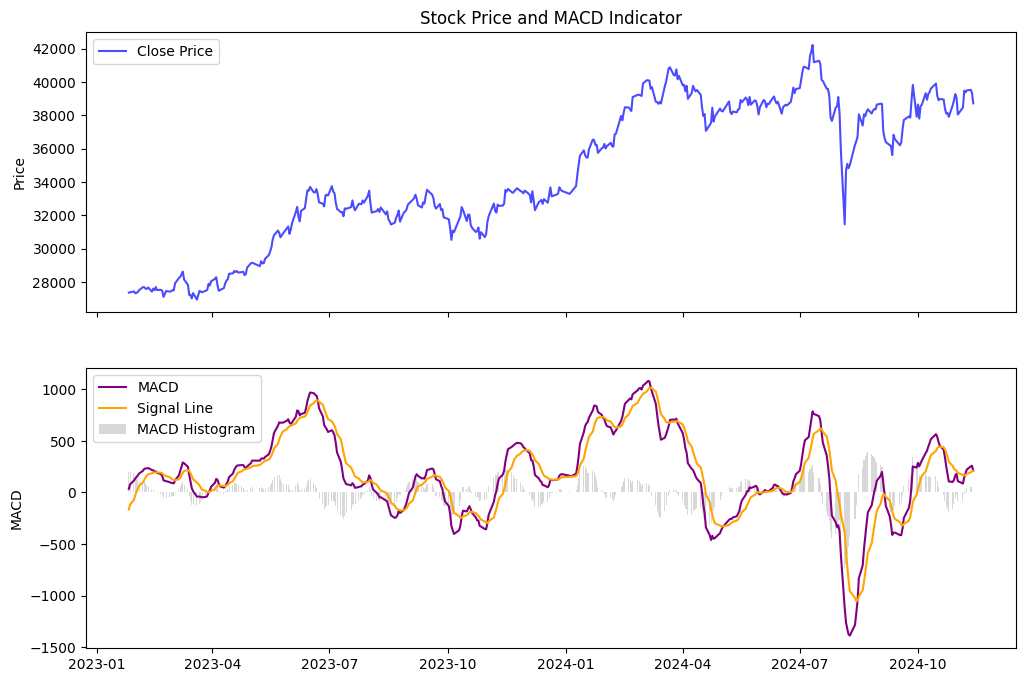
The MACD is a line that fluctates above and below 0 that indicates when the moving averages are converging, crossing, or diverging.

# moving average convergence divergence (macd)
data['ema_12'] = data['Close'].ewm(span=12, adjust=False).mean()
data['ema_26'] = data['Close'].ewm(span=26, adjust=False).mean()
data['macd'] = data['ema_12'] - data['ema_26']
data['signal_line'] = data['macd'].ewm(span=9, adjust=False).mean()
data['macd_histogram'] = data['macd'] - data['signal_line']
data = data.dropna()
display(data.tail())

	Open	High	Low	Close	Volume	Dividends	Stock Splits	sma_20	sma_50	ema_20	ema_50	rsi	volatility	momentum	ema_12	ema_26	macd	signal_line	macd_histogram
Date
2024-11-07 00:00:00+09:00	39745.230469	39884.011719	39020.218750	39381.410156	190000000	0.0	0.0	38901.779102	38211.528594	38756.994064	38756.994064	54.412138	0.012271	443.871094	38860.938570	38675.031304	185.907266	169.430036	16.477230
2024-11-08 00:00:00+09:00	39783.449219	39818.410156	39377.871094	39500.371094	159300000	0.0	0.0	38912.899609	38239.331641	38827.791877	38827.791877	54.822500	0.012138	222.410156	38959.312804	38736.167585	223.145220	180.173073	42.972147
2024-11-11 00:00:00+09:00	39417.210938	39598.738281	39315.609375	39533.320312	122700000	0.0	0.0	38920.521094	38264.225625	38894.985061	38894.985061	55.375531	0.012127	152.429688	39047.621652	38795.215935	252.405717	194.619602	57.786115
2024-11-12 00:00:00+09:00	39642.781250	39866.718750	39137.890625	39376.089844	163000000	0.0	0.0	38909.035547	38284.312187	38940.804564	38940.804564	59.646135	0.012092	-229.710938	39098.155220	38838.243632	259.911588	207.677999	52.233589
2024-11-13 00:00:00+09:00	39317.148438	39377.238281	38600.261719	38721.660156	0	0.0	0.0	38849.591016	38291.494766	38919.933668	38919.933668	55.770084	0.012470	-1188.890625	39040.232902	38829.607819	210.625083	208.267416	2.357668

Plot MACD

The MACD histogram shows the difference between the MACD line and the signal line, highlighting momentum shifts and potential trend reversals. The momemntum shifts occur at points where the two lines crossover.

MACD line above signal = potential buying momentum and entering long position
MACD line below signal = potential selling momentum and entering short position

Long position means that you are buying stocks with the intention of profitting from its rising value
Short position means that you are betting on making money from the stocks falling in value.

# Set up the figure and axes for subplots
fig, (ax1, ax2) = plt.subplots(2, figsize=(12, 8), sharex=True)
# Plot the Closing Price
ax1.plot(data['Close'], label='Close Price', color='blue', alpha=0.7)
ax1.set_title("Stock Price and MACD Indicator")
ax1.set_ylabel("Price")
ax1.legend(loc="upper left")
# Plot the MACD and Signal Line
ax2.plot(data['macd'], label='MACD', color='purple', linewidth=1.5)
ax2.plot(data['signal_line'], label='Signal Line', color='orange', linewidth=1.5)
# Plot the MACD Histogram as a bar plot
ax2.bar(data.index, data['macd_histogram'], label='MACD Histogram', color='grey', alpha=0.3)
# Set labels and title for the MACD plot
ax2.set_ylabel("MACD")
ax2.legend(loc="upper left")
# Display the plot
plt.show()

Define Long - Short Signals

data['position'] = np.nan
# define long position(1) when macd crosses above signal line 
data.loc[data['macd'] > data['signal_line'], 'position'] = 1 
# define short position(-1) when macd crosses below signal line 
data.loc[data['macd'] < data['signal_line'], 'position'] = -1 

Use ffill() to carry forward the last signal until a new signal is generated. This means the position will be held until there is a crossover on the signal line

data['position'] = data['position'].ffill()
display(data.tail())

	Open	High	Low	Close	Volume	Dividends	Stock Splits	sma_20	sma_50	ema_20	ema_50	rsi	volatility	momentum	ema_12	ema_26	macd	signal_line	macd_histogram	position
Date
2024-11-07 00:00:00+09:00	39745.230469	39884.011719	39020.218750	39381.410156	190000000	0.0	0.0	38901.779102	38211.528594	38756.994064	38756.994064	54.412138	0.012271	443.871094	38860.938570	38675.031304	185.907266	169.430036	16.477230	1.0
2024-11-08 00:00:00+09:00	39783.449219	39818.410156	39377.871094	39500.371094	159300000	0.0	0.0	38912.899609	38239.331641	38827.791877	38827.791877	54.822500	0.012138	222.410156	38959.312804	38736.167585	223.145220	180.173073	42.972147	1.0
2024-11-11 00:00:00+09:00	39417.210938	39598.738281	39315.609375	39533.320312	122700000	0.0	0.0	38920.521094	38264.225625	38894.985061	38894.985061	55.375531	0.012127	152.429688	39047.621652	38795.215935	252.405717	194.619602	57.786115	1.0
2024-11-12 00:00:00+09:00	39642.781250	39866.718750	39137.890625	39376.089844	163000000	0.0	0.0	38909.035547	38284.312187	38940.804564	38940.804564	59.646135	0.012092	-229.710938	39098.155220	38838.243632	259.911588	207.677999	52.233589	1.0
2024-11-13 00:00:00+09:00	39317.148438	39377.238281	38600.261719	38721.660156	0	0.0	0.0	38849.591016	38291.494766	38919.933668	38919.933668	55.770084	0.012470	-1188.890625	39040.232902	38829.607819	210.625083	208.267416	2.357668	1.0

Some notes on random forest classifiers:

Bagging or Bootstrap Aggregating uses replacement. This means that after selecting a smaple from the dataset to put into the training subset, you put it back into the dataset and it can be chosen again for the same subset or a different subset. Each subset can contain duplicate samples and some samples from the original dataset may not even be included in a subset for training.

Pasting is the opposite, i.e. without replacement. Each sample in the subset us unique. Every subset of data used for training is therefore completely unique. Pasting works better with larger datasets.

Build and Train Random Forest Classifier

# define features and target
features = ['macd','signal_line','rsi','sma_20','ema_20','ema_50']
target = 'position'

# prep features and target var 
x = data[features]
y = data[target]

# drop rows with missiing values 
x = x.dropna()
y = y[x.index] # make sure target var matches the features 

# split the data 
x_train, x_test, y_train,y_test = train_test_split(x,y, test_size=0.2,shuffle=True)
# print(len(x_train),len(x_test))

# initialize random forest classifier 
rf_model = RandomForestClassifier(max_depth = 10, min_samples_leaf=5, n_estimators=100, random_state=42,oob_score=True)
# train the model 
rf_model.fit(x_train,y_train)

# make predictions on the test set 
y_pred = rf_model.predict(x_test)
# evaluate the model 
accuracy = accuracy_score(y_test,y_pred)
print('accuracy: ',accuracy)
print('classification report: ')
print(classification_report(y_test,y_pred))
print('confusion matrix: ')
print(confusion_matrix(y_test,y_pred))

accuracy:  0.9438202247191011
classification report: 
              precision    recall  f1-score   support

        -1.0       0.96      0.87      0.92        31
         1.0       0.93      0.98      0.96        58

    accuracy                           0.94        89
   macro avg       0.95      0.93      0.94        89
weighted avg       0.94      0.94      0.94        89

confusion matrix: 
[[27  4]
 [ 1 57]]

# check oob score, becuase random forest classfiier immediately creates this as a validation set 
print(rf_model.oob_score_)

0.884180790960452

Random Forest using oob (out of bag) sampling inherently instead of requiring a validation set to be created.

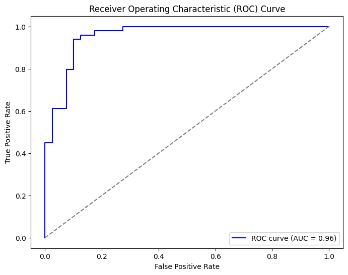
Plot ROC and Calculate AUC

# predict probabilities for the positive class 
y_probs = rf_model.predict_proba(x_test)[:,1]
# calculate roc curve 
fpr, tpr, thresholds = roc_curve(y_test, y_probs)
# calculate auc 
roc_auc = roc_auc_score(y_test, y_probs)

plt.figure(figsize=(8, 6))
plt.plot(fpr, tpr, color='blue', label=f'ROC curve (AUC = {roc_auc:.2f})')
plt.plot([0, 1], [0, 1], color='grey', linestyle='--')  # Diagonal line for random performance
plt.xlabel('False Positive Rate')
plt.ylabel('True Positive Rate')
plt.title('Receiver Operating Characteristic (ROC) Curve')
plt.legend(loc='lower right')
plt.show()

Hyperparameter Tuning

Using default hyperparmeters, I achieved an accuracy score of about 83% which isn’t bad, but can be better. Hyperparameter tuning will search a series of parameters to figure out which ones are the best.

The results show that the best parameters are: max_depth=10
min_samples_leaf=5
n_estimators=25

I went back and replaced the default hyperparameters with the above, but found that when n_estimators = 100, the reuslts were better.

# set the parameters that we want to search 
params = {
    'max_depth': [2,3,5,10,20],
    'min_samples_leaf': [5,10,20,50,100,200],
    'n_estimators': [10,25,30,50,100,200]
}

grid_search = GridSearchCV(estimator=rf_model,
                           param_grid=params,
                           cv = 4,
                           n_jobs=-1, verbose=1, scoring="accuracy")
grid_search.fit(x_train, y_train)

Fitting 4 folds for each of 180 candidates, totalling 720 fits
CPU times: user 2.18 s, sys: 331 ms, total: 2.51 s
Wall time: 29.9 s

GridSearchCV(cv=4,
             estimator=RandomForestClassifier(max_depth=10, min_samples_leaf=5,
                                              oob_score=True, random_state=42),
             n_jobs=-1,
             param_grid={'max_depth': [2, 3, 5, 10, 20],
                         'min_samples_leaf': [5, 10, 20, 50, 100, 200],
                         'n_estimators': [10, 25, 30, 50, 100, 200]},
             scoring='accuracy', verbose=1)

In a Jupyter environment, please rerun this cell to show the HTML representation or trust the notebook.
On GitHub, the HTML representation is unable to render, please try loading this page with nbviewer.org.

Plot Feature Importance

feature_importance = rf_model.feature_importances_
plt.barh(features, feature_importance)
plt.xlabel('Feature Importance')
plt.title('Random Forest Feature Importance')
plt.show()

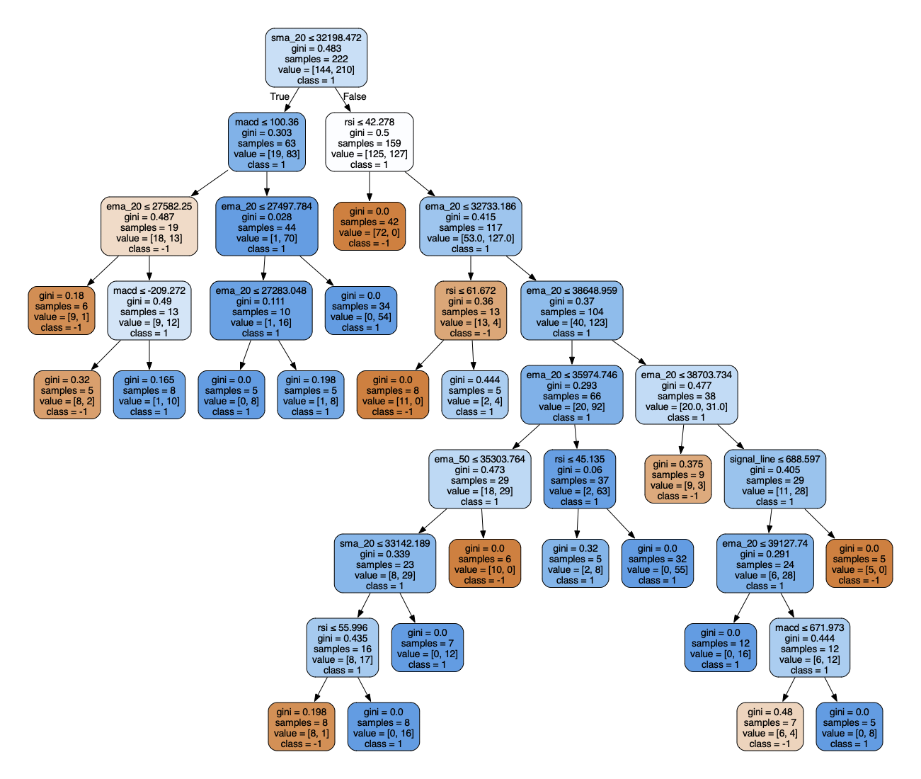
# visualize one of the classifiers 
dot_data = export_graphviz(rf_model.estimators_[0], 
                             out_file=None, 
                             feature_names = x.columns, 
                             class_names=['-1','1'],
                             filled=True,
                             rounded=True,
                             special_characters=True)

graph = graphviz.Source(dot_data)
graph.render("decision tree",format='png',cleanup=True)
graph.view()

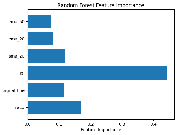
So we can see that the relative strength index is the most important feature in the dataset.

The diagram below shows how the model uses different features and indicates the split rules for all features. Under the label value for each node, the diagram shows the number of samples that were used and the number of samples from each class, where value = [x,y] corresponds to -1,1. In the last line of the node, the class value shows teh most common class.

Generate Predictions

Finally, we can generate predictions on the entire data set and compare the predicted positions with the actual positions.

data['predicted_position'] = rf_model.predict(x)
final = data[['position', 'predicted_position']]
display(final)

	position	predicted_position
Date
2023-01-26 00:00:00+09:00	1.0	1.0
2023-01-27 00:00:00+09:00	1.0	1.0
2023-01-30 00:00:00+09:00	1.0	1.0
2023-01-31 00:00:00+09:00	1.0	1.0
2023-02-01 00:00:00+09:00	1.0	1.0
...	...	...
2024-11-07 00:00:00+09:00	1.0	1.0
2024-11-08 00:00:00+09:00	1.0	1.0
2024-11-11 00:00:00+09:00	1.0	1.0
2024-11-12 00:00:00+09:00	1.0	1.0
2024-11-13 00:00:00+09:00	1.0	1.0

443 rows × 2 columns

We can also see where the actual, calculated decision does not match the predicted position.

display(data.loc[data['position'] != data['predicted_position']])

	Open	High	Low	Close	Volume	Dividends	Stock Splits	sma_20	sma_50	ema_20	...	rsi	volatility	momentum	ema_12	ema_26	macd	signal_line	macd_histogram	position	predicted_position
Date
2023-02-17 00:00:00+09:00	27484.599609	27608.589844	27466.609375	27513.130859	68800000	0.0	0.0	27467.344141	27015.462773	27385.025950	...	52.544581	0.005926	959.601562	27507.998171	27317.894436	190.103735	194.787100	-4.683365	-1.0	1.0
2023-02-20 00:00:00+09:00	27497.130859	27531.939453	27426.480469	27531.939453	62500000	0.0	0.0	27498.639160	27012.373555	27399.017712	...	56.923727	0.005276	625.900391	27511.681445	27333.749623	177.931823	191.416045	-13.484222	-1.0	1.0
2023-03-30 00:00:00+09:00	27827.890625	27876.380859	27630.550781	27782.929688	82000000	0.0	0.0	27684.621777	27494.761758	27570.491005	...	38.133818	0.011013	266.400391	27576.015957	27556.687718	19.328239	6.294103	13.034136	1.0	-1.0
2023-04-10 00:00:00+09:00	27658.519531	27737.490234	27597.179688	27633.660156	48000000	0.0	0.0	27573.137891	27619.602656	27687.528395	...	62.826132	0.010656	-510.310547	27711.332896	27663.756052	47.576844	63.484004	-15.907160	-1.0	1.0
2023-04-11 00:00:00+09:00	27895.900391	28068.390625	27854.820312	27923.369141	64800000	0.0	0.0	27577.658301	27630.418828	27709.989418	...	59.318753	0.010660	90.408203	27743.953857	27682.986651	60.967206	62.980644	-2.013439	-1.0	1.0
2023-09-21 00:00:00+09:00	32865.558594	32939.890625	32550.650391	32571.029297	107900000	0.0	0.0	32713.799609	32494.285820	32757.701448	...	49.321868	0.010014	560.769531	32873.815310	32694.564731	179.250579	169.147336	10.103243	1.0	-1.0
2023-10-16 00:00:00+09:00	31983.039062	31999.789062	31564.310547	31659.029297	84500000	0.0	0.0	32080.802930	32235.168242	31981.839379	...	40.252909	0.013162	-1509.072266	31870.004290	32053.219943	-183.215653	-221.515003	38.299350	1.0	-1.0
2023-10-25 00:00:00+09:00	31302.509766	31466.919922	31195.580078	31269.919922	78700000	0.0	0.0	31597.691309	32122.819609	31678.628901	...	57.970678	0.013278	-1045.130859	31506.207344	31778.585800	-272.378456	-225.425469	-46.952987	-1.0	1.0
2023-11-01 00:00:00+09:00	31311.220703	31601.650391	31301.509766	31601.650391	130100000	0.0	0.0	31380.244824	32044.875977	31406.949473	...	40.677205	0.014841	363.710938	31228.198012	31523.362572	-295.164560	-295.774575	0.610016	1.0	-1.0
2023-12-04 00:00:00+09:00	33318.070312	33324.378906	33023.039062	33231.269531	87300000	0.0	0.0	33115.909180	32218.798789	33032.855349	...	63.357467	0.009593	1281.378906	33265.644680	32885.774493	379.870187	404.636944	-24.766757	-1.0	1.0
2023-12-26 00:00:00+09:00	33295.679688	33312.261719	33181.359375	33305.851562	68300000	0.0	0.0	33080.057227	32578.252500	33076.413488	...	48.296399	0.011044	-102.539062	33145.258185	33015.601761	129.656424	125.346315	4.310109	1.0	-1.0
2024-01-30 00:00:00+09:00	36196.640625	36249.031250	36039.308594	36065.859375	87900000	0.0	0.0	35215.043555	34015.763125	35337.236029	...	69.772308	0.009780	2384.621094	35774.784950	35050.490528	724.294422	730.132578	-5.838156	-1.0	1.0
2024-03-08 00:00:00+09:00	39809.558594	39989.328125	39551.601562	39688.941406	143300000	0.0	0.0	38830.578320	36628.270859	38809.261927	...	71.310158	0.010562	3569.019531	39377.822010	38399.300401	978.521609	1009.610745	-31.089136	-1.0	1.0
2024-03-25 00:00:00+09:00	40798.960938	40837.179688	40414.121094	40414.121094	101500000	0.0	0.0	39601.740430	37836.404219	39429.966488	...	53.418080	0.011011	1315.441406	39827.164290	39119.040156	708.124134	686.521700	21.602435	1.0	-1.0
2024-03-26 00:00:00+09:00	40345.039062	40529.531250	40280.851562	40398.031250	101400000	0.0	0.0	39659.956445	37943.367656	39522.163132	...	53.364377	0.011013	1164.320312	39914.989976	39213.780237	701.209739	689.459308	11.750432	1.0	-1.0
2024-03-27 00:00:00+09:00	40517.171875	40979.359375	40452.210938	40762.730469	121300000	0.0	0.0	39736.116992	38047.080078	39640.312402	...	56.967091	0.011133	1523.210938	40045.411590	39328.517291	716.894299	694.946306	21.947993	1.0	-1.0
2024-05-30 00:00:00+09:00	38112.769531	38138.031250	37617.000000	38054.128906	117300000	0.0	0.0	38561.450195	38971.007187	38604.989942	...	47.636190	0.008827	-351.531250	38606.600319	38616.011877	-9.411558	1.325213	-10.736770	-1.0	1.0
2024-05-31 00:00:00+09:00	38173.218750	38526.929688	38087.609375	38487.898438	211000000	0.0	0.0	38572.142578	38945.956328	38593.838370	...	53.774913	0.009177	213.847656	38588.338491	38606.521993	-18.183501	-2.576530	-15.606971	-1.0	1.0
2024-10-18 00:00:00+09:00	39092.468750	39186.640625	38893.519531	38981.750000	95700000	0.0	0.0	38726.598047	37697.068047	38707.127747	...	44.308282	0.018217	2601.578125	38996.177299	38542.783793	453.393506	444.418413	8.975093	1.0	-1.0
2024-11-06 00:00:00+09:00	38677.949219	39664.531250	38662.171875	39480.671875	170600000	0.0	0.0	38879.585547	38191.185781	38691.266054	...	52.731370	0.012487	147.933594	38766.307372	38618.520996	147.786377	165.310729	-17.524352	-1.0	1.0

20 rows × 21 columns